Google Sheets: The 2022 Most Complete Guide

Spreadsheets offer a whole new way of handling and analyzing any information. That’s why people use Microsoft Excel so much. But since Google Workspace has become so popular these days, many professionals and individuals migrate to Google Sheets. Mainly because it is a free tool that you can use online. Needless to say, the list of benefits of a tool with these characteristics goes on and on.

Some people may question if Sheets is as good as Excel, if it does the same things, and accepts the same formulas… And the answer is yes! It does. It has so many features, and it is as useful as the other spreadsheet programs available on the market.

This complete guide will lead you towards the best use of Google Sheets and convince you that migrating to this tool will be very satisfactory.

What is Google Sheets and why use it?

Google Sheets is part of G Suite, and it is a web-based free spreadsheet program, like the other software included in this suite. This means you produce your spreadsheets inside your web browser and not as a common software installed on your computer.

As a G Suite app, Google Sheets has the same aspects the other apps do: collaboration, personalization, auto-save, and on and off editing. In short, these are the reasons why you should migrate to this tool.

Work online (and offline too)

One thing that makes Google Sheets different from its big competitors is the cloud-based aspect. When you can edit something online, you eliminate the needing for storage in your computer, reduce precious time and steps on the collaborative edition and give mobility to handle data.

First, if you don’t have to install software on your computer, you save space in your HD. And as the spreadsheets are saved in the cloud, it’s unnecessary to keep them on your computer if you don’t want to.

Second, you can edit your spreadsheets with teammates in real-time to facilitate the work and avoid serious mistakes. We will talk more about it later, and you will learn how to use this feature in the best way possible.

Last but not least, you have the chance to access your spreadsheets anywhere you go, on any device, even the ones that you don’t own. You have to log in with your Google account and choose the file.

On the other hand, you can also edit your spreadsheets even when you don’t have internet available. By installing this Chrome extension, you can edit your data offline. After the installation, choose the tab “File” on the menu bar and click on “Make available offline.” 

Another option is downloading the file and editing it on other spreadsheet software, such as Excel or Libre Office Calc. 

Auto-save

Every time you stop to perform a simple action in your spreadsheet, Google Sheets automatically saves it. It’s an auto-save tool that is doing its job every second of the edition. Therefore, it eliminates the need to hit the save button, which doesn’t exist in Google Suite apps.

Collaboration in real-time

One of the best features of Google Sheets is collaboration in real-time. It’s an essential characteristic that teams can benefit from. 

There are three collaborative elements that Google Sheets offer: Comments, Share, and Edit.

Comments

This resource is used a lot when you are editing a spreadsheet simultaneously with other teammates. Some actions can be adding notes and commenting suggestions, calling attention to specific data in the spreadsheet. To add a comment, you can click on a cell or select a range of cells. Hover the selection, then click with the mouse’s right button, choosing the option “Comment.” It’s also possible to press the keyboard shortcut Ctrl+Alt+M.

The comments are displayed in boxes on the selection side, with the name and photo of the person who commented. It’s an interactive box where you can reply and mention someone that needs to act, and collaborators can reply to them. After making the necessary actions requested on the comments, click on “Resolve” to make a comment disappear. 

Share

Forget about losing time, sending common spreadsheets via email to your teammates. Besides this huge problem, every time you share an offline spreadsheet, it generates countless versions edited by each person. Both processes can become a real mess.

With Google Sheets, you can share your spreadsheets with your team, and they can view or edit it online.

To share a spreadsheet, access the tab “File,” then “Share.” A popup will open with a type box to enter the email addresses of the people you want to share with. On the top right of the popup, you can also click on “Get Shareable Link” to share the link directly with your teammates via other communication channels. In this popup, you can also set up the privileges you want to give to them: view, comment, or edit.

Beginning with View, which allows visualization of the spreadsheet in real-time. The second is Comment that brings the possibility to view and add comments over the spreadsheet. And at last, Edit, that gives full permission to whom you are sharing it with.

If you feel the need to restrict your spreadsheet access, choose the option “Advanced,” then click on “Prevent editors from changing access.” This way, you override the chance of your data being shared with people you don’t want to have access to.

If you want to see who has access to your spreadsheet and delete access to them, you can also do that in the advanced options.

Edit

To eliminate the dozens of versions generated by sending the spreadsheets, edition in real-time is a great alternative that Google Sheets offers. This solution saves a lot of time, and it’s practical because up to 50 people can access and edit spreadsheets simultaneously. Therefore a big team will certainly benefit from this feature. 

To better use, this edition, the comments and the chat in real-time are complementary tools that avoid miscommunication and mistakes.

Personalize your Google Sheets

 

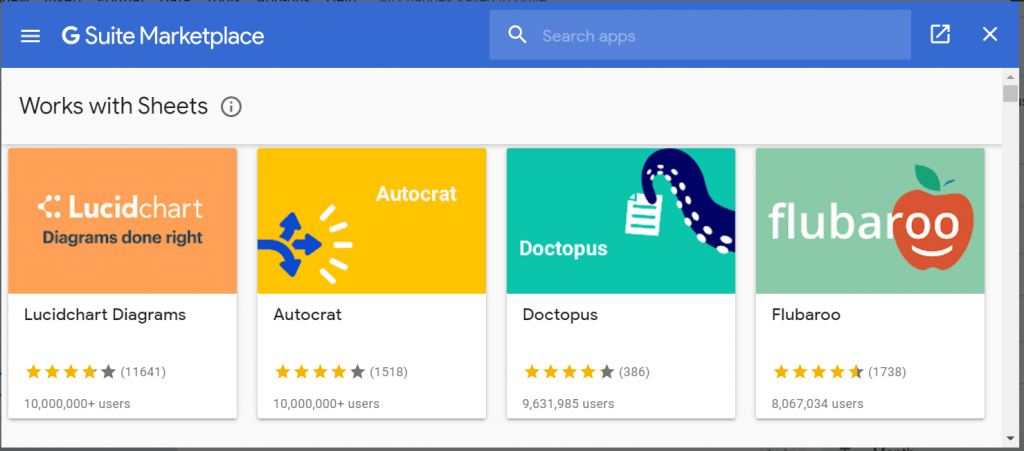Each individual, or team, has its methods and processes while working with spreadsheets. That’s why you can personalize the experience inside Google Sheets, using elements like Add-ons.

Some Add-ons help you build diagrams, change table styles, get data from outside software, and so on.

To see the available ones, click on Add-ons in the menu bar and then “Get Add-ons.” A G Suite Marketplace popup will open with a search bar and the featured add-ons that work with Google Sheets. Choose those that will facilitate your life dealing with spreadsheets, making sense of the type of business you have.

Google Sheets terms

To fully understand how to use Google Sheets, you must be familiarized with common terms that you will find on this software because sometimes errors and warnings may appear, and you know how to deal with them knowing these terms.

• Cell: Spreadsheets are made with lots of cells. That rectangular box resulted from a vertical column’s intersection, and a horizontal row is called a cell. 
• Row: Rows are the horizontal lines of cells. Numbers represent them from 1 to infinite. Therefore you can have spreadsheets of the size you need.

 

• Column: Columns are the vertical series of cells. Each one of them is represented by a letter. Despite that, as the rows, they can also be infinite. After the letter Z, the letters start becoming AA, AB, AC, and so on.

 

• Range: It’s a group of selected cells. The range can be across a column, row, or both. 

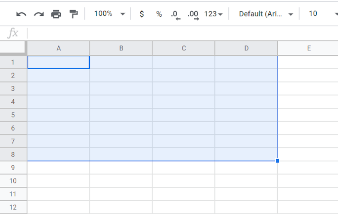
• Array: It’s a range but used in a formula. 
• Function: The operations that you can use to calculate values, manage data. There is a function/formula bar between the spreadsheet grid and the toolbar. There is a function/formula bar (with the “fx” symbol). This space is used to type formulas, functions, text, etc.

 

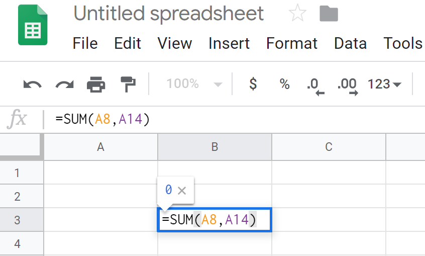
• Formula: To generate a result, we use formulas that combine functions, rows, cells, columns, and ranges.

How to Use Google Sheets the best way

After knowing the main terms of Google Sheets, it is time to learn how to use it properly. In fact, when you know each one of the elements, tools, and functionalities, you can improve your experience inside this online software.

Toolbar

First things first, you need to be familiarized with the toolbar’s icons, so you can save time while editing your spreadsheets. This happens because you are taking shortcuts while using the toolbar directly, and not those infinite paths and clicks to get things done. There are 28 tools available on the Sheets toolbar, and we are going to figure out each one of them:

• Undo: Represented by the curved arrow to the left helps correct any mistake you have made and restore immediate editions. 
• Redo: If you have undone something and want it back, click this button, represented by a curved arrow to the right.
• Print: Click on this symbol to print your spreadsheet. It’s a faster method than going to “File” then clicking on “Print.”
• Paint Format: If you want to easily set a format to your cells, select the cell or ranges of cells with the desired format. Then click on Paint Format to copy it. After this, the cursor will turn into a paint roller, and you can select the part of the spreadsheet you want to format.
• Zoom: It controls the size you display your document. For instance, when you need to see a cell in detail, you can zoom in to visualize it bigger.
• Format (as currency ($) and as a percentage(%): Ideal to format a range quickly with a currency or percentage. 
• Decrease and Increase decimal places: Two buttons that can speed the process of changing the decimal position.
• More Formats: Here, you can see all the formats you can use in your data, including time, date, accounting, and others.
• Font: Choose the font style according to your needs.
• Font Size: Control the size of your font.
• Bold (B), Italic (I), Underline (U): Highlight your texts inside the spreadsheet with these styles
• Text Color: Change the color of your text to any existing color.
• Fill color: Fill your cells or ranges of cells with color. It’s a useful tool for tables because it facilitates viewing and organizing content.
• Borders: Choose how the borders will be, their color, and their style.
• Merge Cells: This tool only becomes available when you select a range. You can merge two or more cells.
• Align: You can align the data inside the cells to the left, center, or right.
• Vertical align: Align the position of your data to the top, center, or bottom of the cell.
• Text Wrapping:  There are three possibilities of text wrapping inside Google Sheets (Overflow, Wrap, and Clip). They will basically help you display your text inside a cell or beyond the boundaries of a cell.
• Text Rotation: Sometimes, you need to display data differently. That’s why this tool gives you the possibility of rotating the cell’s content from different angles.
• Insert Link: Select the word or sentence you want to be clickable and redirect to a certain URL. Then click on this symbol ( paper clip) and paste the URL in the popup.
• Insert comment: This is a useful tool for collaboration inside the spreadsheet. Select the cell or range you want to add a comment.
• Insert chart: If you work with charts, this button will be essential to you. Select the desired range of data you want to turn into a chart, then click on this button. A Chart Editor box will appear, and you will be able to set everything the way you need.
• Create a filter: A fast and easy way to start creating new filters.
• Functions: Here, you can see a drop-down list with the most used functions, such as SUM, AVERAGE, and COUNT. You can also choose from a list separated by categories (Math, Date, Engineering…) or see all of them. This is helpful to insert the function, so you don’t need to memorize all of them.

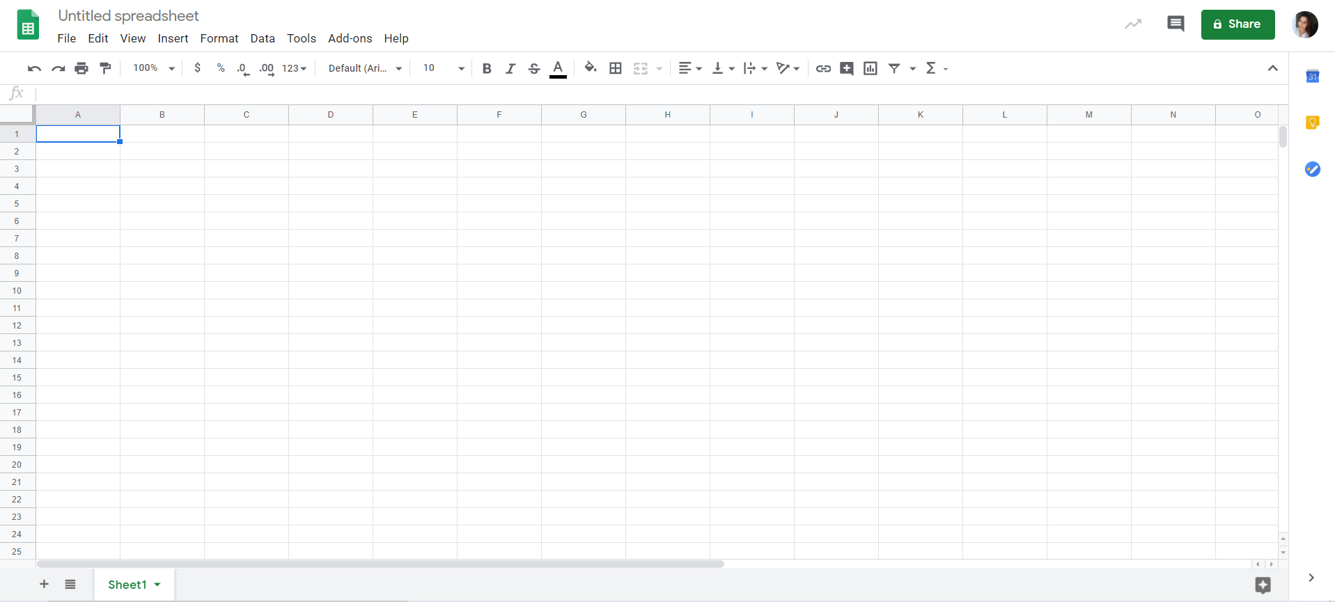
How to Create a New Spreadsheet

To create a new spreadsheet, you have two options. The first one is to access the Google Sheets site and choose “Blank” represented by the plus symbol if you want to start from scratch. You can also choose a template to save you time, such as Invoices, Expense reports, monthly budgets, to-do lists. And the list goes on and on with nice templates to help you with the design aspect of a spreadsheet. 

The other way is when you are already inside a spreadsheet and want to open a new one. Just click on “File,” then on “New” and  “Spreadsheet.”

Protecting Your Data

Some sheets may have confidential data that needs to be protected. Google Sheets allows you to that by following the steps:

 Click on “Data” > “Protected Sheets and Ranges.”

• Then choose between “Range” to protect a specific range of cells or “Sheet” to protect the entire spreadsheet. If you chose the first one, select the range of cells you desire to protect.
• Next, click on “Set Permissions,” then choose to display a warning to those who intend to edit or customize editing permissions for certain people.

How to Hide and unhide Data

Additionally, you can protect your data by hiding it. Sometimes you need to restrict data views while sharing your spreadsheet, so Google Sheets also thought about adding this feature.

To hide a column, click with the mouse’s right button on this column, and then select the option “Hide Column.” Note that two arrows will appear in the columns between the one you hid. 

On the other hand, to unhide the column, hover over one of these arrows, then other arrows in a white box will appear. You can click on either of them to display the column again.

 

You can also use this resource when you want to control the data you’re viewing at a time. As we said before, spreadsheets can have so much information that it’s necessary to use some resources to view the content better. And this is one of the best resources.

Using filters to organize data

For starters, spreadsheets can have so much information that it may be hard to find what you need. That’s why Google Sheets has numerous filters that will help you display only what you want to see.

If you need to view data in a single column with specific criteria, for example, all the negative numbers on a table of financial content, you can apply a filter to do it. Or imagine you need to see all the cells that contain the industry your clients belong to, such as “Real Estate.”

To do the filtering process, start by selecting the column(s) you want to filter and then select “Data” on the menu bar. Then choose “Create a Filter.” Click on the funnel icon that will appear in the column, where you can choose to filter by value, condition, alpha, or numeric order. This way, the spreadsheet will only show data that fits the criteria you have applied.

Edit Excel sheets in Google Sheets

Yes, you can edit Excel Sheets in the Google free software! Just import the file following this path: Go go to “File,” then click on “Import,” choosing “Upload” next. Please select the file you want to import, being aware that you must save it in file formats that don’t require password protection, such as .csv, .xls, and others.

After that, the Excel sheet will be converted to a Google sheet.

Google Sheets advanced tips

Now that you are familiar with the basics of Google Sheets, how about level up and start learning more advanced tips?

Macros

This feature offers the possibility to store a command sequence or function on a VBA module. Therefore you can use it to perform a task, like a shortcut. It’s commonly used for repetitive tasks to avoid loss of time and long processes.

Start creating your macros by going to “Tools,” then “Macros.” Choose the option “Record macro,” manage or import the existing ones.

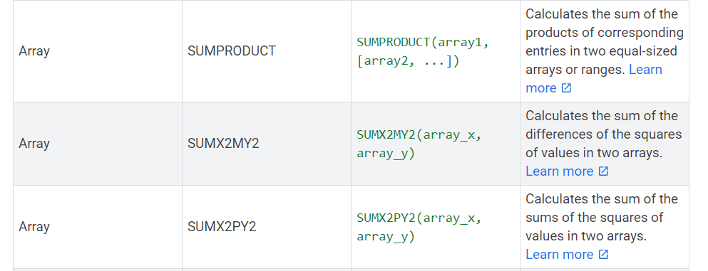
Array Formulas

According to Google, an array formula is “a formula that can perform multiple calculations on one or more items in an array.” It’s a way to make the calculation inside your spreadsheet more efficient, mainly when it has a huge amount of data. Check some examples of array formulas below:

Creating graphs

Displaying data in charts is one of the most used tools in the business context. That is the reason why it is so important to learn how to create them inside Google Sheets. Go through the following steps:

1. Select the range of data you desire to transform in a chart. If you want to pre-label the chart, add a header row or column.
2. Next, click on “Insert,” then on “Chart.”
3. A side panel will open, then you have to choose the option “Data,” which is under “Chart type.” Next, choose a chart. 
4. To personalize your chart style, text, and colors, click on “Customize.”

How to Create a Pivot Table

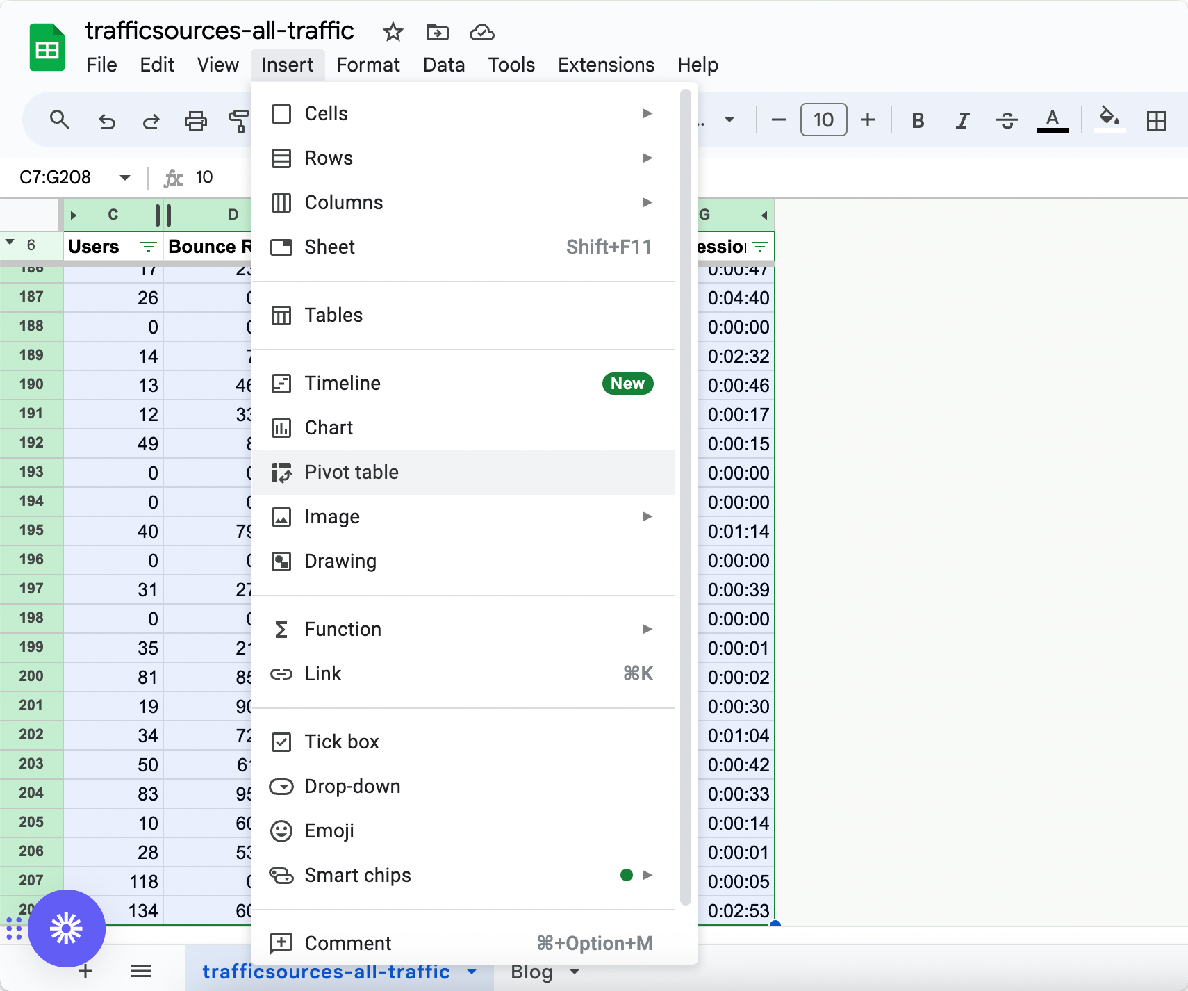A Pivot Table is an advanced tool to calculate, summarize, and analyze data. It allows you to see patterns, trends, and comparisons in your data. 

Follow these steps to create your pivot table in Google Sheets:

1. First, select the cells with data you want to use in your pivot table. Notice that each column needs a header.
2. Next, click on “Data” in the menu bar and choose the “Pivot table.” Then click the pivot table sheet if it’s not open yet. 
3. In the side panel, next to “Rows” or “Columns,” click “Add” and choose a value. To add an existing pivot table, under “Suggested,” select it.
4. Still in the side panel, click “Add” next to “Values.” After, choose the value you desire to display in your rows or columns.
5. If you want to change something, click the down arrow next to it. 

Translate without leaving your Google Sheet

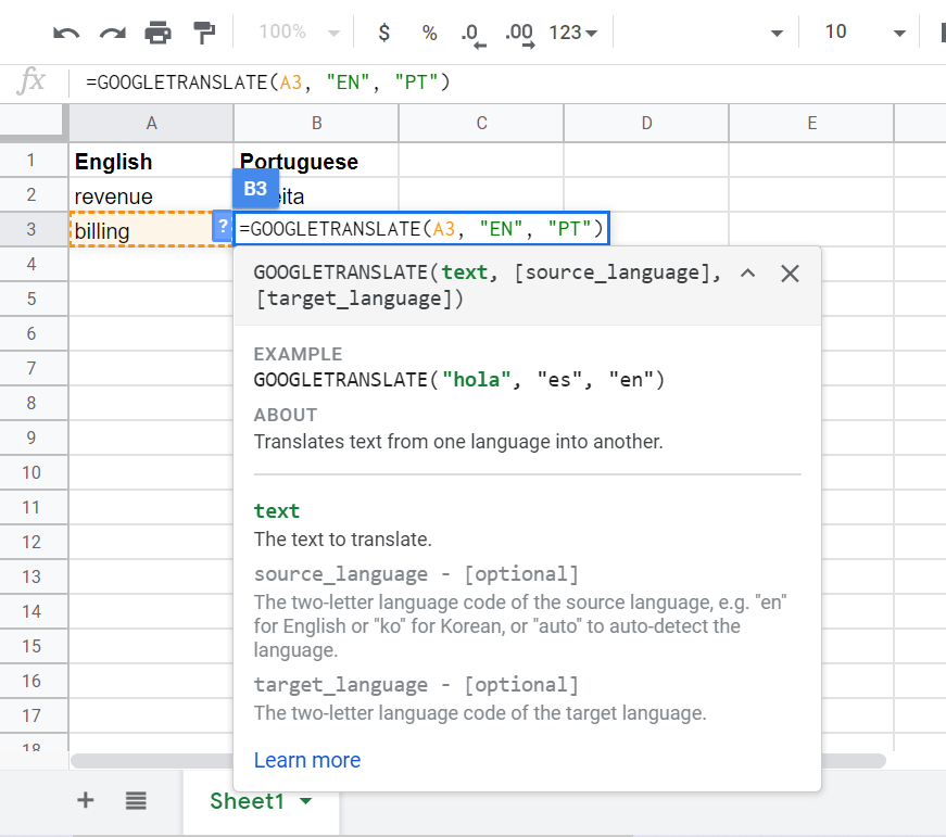If you need to work with Sheets in another language, you can save time by using this function: GOOGLETRANSLATE. It will translate all values into a different language. Simple and útil, cierto?

10 Google Sheets Formulas you should know

Many times you need to get quick results inside a spreadsheet. That’s why people use formulas for almost everything. It facilitates your work one hundred percent because you don’t need to worry about calculating by yourself. So check the 10 most commonly used Google Sheets formulas, and learn how to deal with your data the best way possible.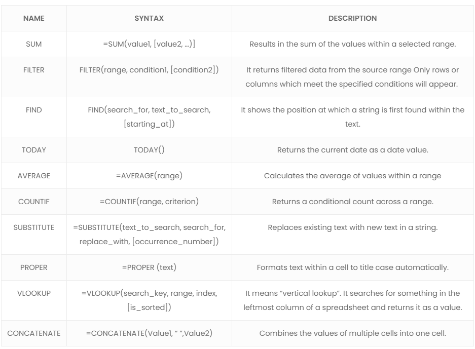

There are lots of formulas you can use besides these. Check them out on the Google Sheets function list. They are divided into categories: Array, Database, Date, Engineering, Filter, Financial, Google, Info, Logical, Lookup, Math, Operator, Statistical, Text, Parser, and web.

Summarizing

It’s always good to have an alternative that fits all your needs. Better yet, if it is a free one, that has countless benefits. 

So, if you are part of a team, Google Sheets is the best choice of a spreadsheet program for you, mainly because of its collaboration features.

Briefly, we hope to see you applying the basic and advanced tips and tricks we have presented so that you can handle your spreadsheets way better than before.